Animation with GNUPlot
An Introduction to visulaization of Physical system
By, Arabindo on 9th Oct, 2021 Comments
For any error/mistakes feel free to contact me at arabindo@pm.me
Home | Prev. Page | Resources
Content
- 1.Introduction 2. The ‘Hellow World!’ 3. Working Equations 4. Phase space 5. Final code 6. Appendix-I(Derivations)
Introduction
Here we are at the very end of this animation blog. Now we are equipped with a lot of features of GnUPlot. The last thing I wanted to show, how to animate from a dat or txt file. You may be able to plot a static graph from files but animating from a file requires reading data line by line. at first, we will go through a simple example, which will show all the essence of ‘animation from a data file’ then we will move on to simulate Kapitza Pendulum.
The ‘Hello World!’ - Once Again
Here I have generated a data file ‘data_gen.dat’ using a Fortran program. You may see it here.
The code for GNUPlot is simple and self-explanatory ~
reset
set term qt
unset key
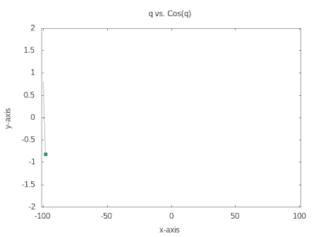
set title 'Test'
set xlabel 'x-axis'
set ylabel 'y-axis'
set yrang[-2:2]
set xrange[-101:101]
n=2000
do for[i=1:n]{
plot 'test.dat' every ::1::i w l ls 1, \
'test.dat' every ::i::i pt 5
}
reread
In the plot command, first line is meant to plot from the first line of data_gen.dat upto \(i^{th}\) line. The output must explain the need. The second line of plot is the point which is guiding the curve in this GIF.
Working Equations for Kapitza Pendulum
The Lagrangian is \[ L = \frac{m}{2}\left[ z_0^2 \omega^2 sin^2 (\omega t)+l^2 \dot{\theta}^2 + 2z_0 l \omega \dot{\theta} sin(\omega t) sin \theta \right] - mg\left( z_0 cos(\omega t) + l cos\theta \right) \]
Then it’s easy to show, ( Details are here ) the equation of motion is: \[ \ddot{\theta} + \frac{sin \theta}{l} \left( z_0 \omega^2 cos (\omega t) - g \right) \]
As we’ve done before
\[ \dot{\theta} =\Theta \] \[\dot{\Theta} = -\frac{sin \theta}{l} \left( z_0 \omega^2 cos (\omega t) - g \right)\]
Here, \(z = z_0 cos (\omega t)\), z is the coordinate of the base while \(\omega\) is the frequency. \(\theta\) is the angle between baseline and pendulum. \(l\) is the length of the pendulum.
The Fortran code to solve the equations can be found here. You may just download the generated file.
Look at phase space
Before we simulate the Pendulum itself, let us simulate the phase space portrait. One can always do a static plot p 'kp.dat' u 2:3 w l
But it’s boring. In the previous example, we’ve seen how to do animation from data files. So you may try it yourself. Although I’m leaving the code that creates a GIF for you. This code may take longer in the first run as the number of frames is large.
The Kapitza Pendulum
Here, we not only need to read the data line by line from the file but also need to store them in variable since we need them to use in drawing bobs and anchor, as we have done before. For this, I did a little trick here. I’ve plotted first and second column with white colour(see line no. 44), meanwhile, store them into variable. The output will look like as the cover of this page. So, here we go~
Configuration Space
You may try to plot configuration space as well! That is column 1 vs Column 2.
Appendix-I (Derivations)
For the derivation of Lagrangian and EOM, you may check out my blog post on Kapitza pendulum
Home | Prev. Page | Resources