Lagrangian Dynamics of Kapitza's Pendulum and It's Numerical Solution
Kapitza’s Pendulum is nothing but a regular pendulum which is inverted and pivoted to a oscillator. Interestingly, When the frequency of the oscillator is very high, the pendulum doesn’t fall down. Here we seek for the equation of motion and numerical solution for such system.
Here the generalised coordinate is \(\theta\)(q in the diagram). The pendulum has a length \(l\). The base point of the pendulum is oscillating with a frequency \(\omega\) and amplitude is \(z_0\).
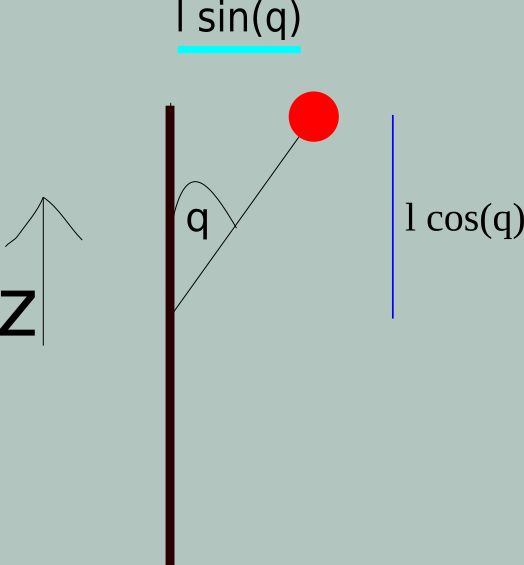
Therefore, the equation for the base point maybe written as \(Z = z_0 \cos\omega t \) (We used capital Z for a reason, will be clear in a minute)
From the pictorial description, for the bob, we have \(z = Z + l\cos\theta \) and \( x= l\sin\theta \)
The kinetic energy term is :
\[\begin{eqnarray} T &=& \frac{1}{2}m(\dot{z}^2 + \dot{x}^2) \\ \implies T &=& \frac{1}{2}m[z_0 ^2 \omega^2 \sin^2\omega t + l^2\dot{\theta}^2 \sin^2 \theta + 2z_0\omega l \dot{\theta} \sin\omega t \sin\theta + \dot{\theta}^2 \cos^2 \theta] \tag{1} \end{eqnarray}\]Potential energy term is \[U = mg(Z + l\cos\theta) = mg(z_0 \cos\omega t + l\cos\theta) \tag{2} \]
Therefore the Lagrangian(L=T-U) of the system is given by, \[L = \frac{1}{2}m[z_0 ^2 \omega^2 \sin^2\omega t + l^2\dot{\theta}^2 + 2z_0\omega l \dot{\theta} \sin\omega t \sin\theta] - mg(z_0 \cos\omega t + l\cos\theta) \tag{3} \]
The Equation of Motion[EOM] is, \[\frac{d}{dt}\left(\frac{\partial L}{\partial\dot{\theta}}\right) - \frac{\partial L}{\partial \theta} = 0 \] \[\implies l^2 \ddot{\theta} + z_0l\omega^2\cos{\omega t}\sin\theta + z_0l\omega\dot{\theta}\sin{\omega t}\cos\theta - z_0l\omega\dot{\theta}\sin{\omega t}\cos\theta - gl\sin\theta = 0\] \[\implies \ddot{\theta}+\frac{\sin\theta}{l}\left(z_0 \omega^2 \cos{\omega t} - g \right) = 0 \label{4} \tag{4} \]
For the numerical solution, we need to convert the equation \( \ref{4} \) into two first order equation as follows,
\[\begin{eqnarray} \dot{\theta} &=& \Theta = f_1(\theta, \Theta, t) \\ \dot{\Theta} &=& - \frac{sin\theta}{l}\left(z_0 \omega^2 cos(\omega t) - g \right) = f_2(\theta, \Theta, t) \end{eqnarray}\]For the numerical solution, we would like to apply RK-4 method. The corresponding equations will be,
\[\begin{eqnarray} k_{11} &=& dt \times f_1(\theta, \Theta, t) \\ k_{12} &=& dt \times f_2(\theta, \Theta, t) \\ \\ k_{21} &=& dt \times f_1 \left(\theta + \frac{k_{11}}{2}, \Theta + \frac{k_{12}}{2}, t + \frac{dt}{2} \right) \\ k_{22} &=& dt \times f_2 \left(\theta + \frac{k_{11}}{2}, \Theta + \frac{k_{12}}{2}, t + \frac{dt}{2} \right) \\ \\ k_{31} &=& dt \times f_1 \left(\theta + \frac{k_{21}}{2}, \Theta + \frac{k_{22}}{2}, t + \frac{dt}{2} \right) \\ k_{32} &=& dt \times f_2 \left(\theta + \frac{k_{21}}{2}, \Theta + \frac{k_{22}}{2}, t + \frac{dt}{2} \right) \\ \\ k_{41} &=& dt \times f_1 \left(\theta + k_{31}, \Theta + k_{32}, t + dt \right) \\ k_{42} &=& dt \times f_2 \left(\theta + k_{31}, \Theta + k_{32}, t + dt \right) \\ \\ \theta &=& \theta + \frac{1}{6} \left(k_{11} + 2k_{21} + 2k_{31} + k_{41} \right) \\ \Theta &=& \Theta + \frac{1}{6} \left(k_{12} + 2k_{22} + 2k_{32} + k_{42} \right) \\ t &=& t + dt \end{eqnarray}\]The fortran code to solve the above equation can be found here.
For the animation of the System and phase space, you may checkout my animation blog.